Provenance

When composing processes, it is often necessary to keep track of which component processes own the inputs and outputs (or rather the different parts of the single output) of a composite process. We call this information provenance.

For example, provenance can provide essential metadata to be able to correctly visualize a composite process diagrammatically.

Example

We begin with a motivating example to explain the purpose that provenance fulfils for the visualization of resource-based composition.

Specification

Assume the following process specifications:

• P1: ⊢ NEG X, A ⊗ B
• P2: ⊢ NEG B, C ⊕ D
• Q1: ⊢ NEG A, E
• Q2: ⊢ NEG E, NEG (C ⊕ D), Y

We then perform JOIN operations for each pair, obtaining the following intermediate compositions:

• P: ⊢ NEG X, A ⊗ (C ⊕ D)
• Q: ⊢ NEG A, NEG (C ⊕ D), Y

Finally, we JOIN the 2 results to obtain the final composition:

• R: ⊢ NEG X, Y

Visualization

At the logical level, the composition above seems straightforward. The visualization, however, needs to reveal more information. We need to accurately depict how the individual components are connected to each other, and how resources flow between them.

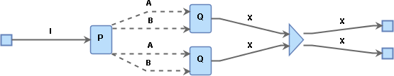
The image below shows the following processes in this order: P1, P2, P, Q, and R.

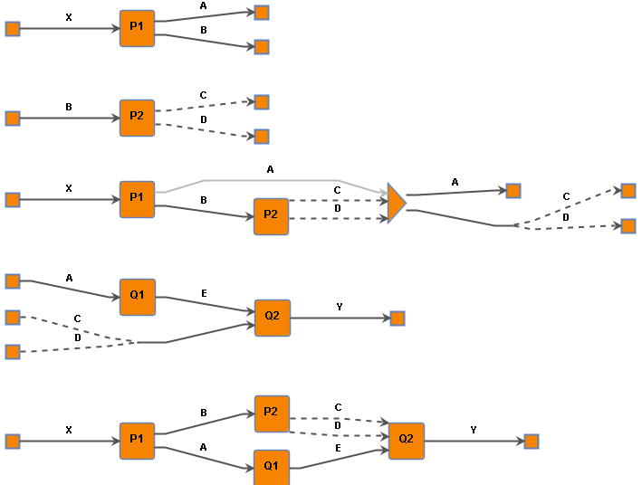
In the visualization of R, the system has inferred that resource A connects P1 to Q1, whereas P2 and Q2 are connected by C ⊕ D. This is achieved despite the fact that the last composition action joined intermediate processes P and Q, meaning the whole term A ⊗ (C ⊕ D) was "cut" in one go.

This is accomplished by tracking the input and output provenance of the involved processes. Specifically, when composing P, we track its output provenance for the output A ⊗ (C ⊕ D) is one where A came from P1 and (C ⊕ D) came from P2. Similarly, when composing Q, we track the input provenance, i.e. that NEG A belongs to Q1 and NEG (C ⊕ D) belongs to Q2. This way, when P and Q are joined, we know exactly where each connected resource is coming from and going to.

Provenance Trees

We want to be able to track provenance of specific CLL resources. This means subterms of the same term can have different provenance. For this reason, we track provenance using a binary tree structure that matches the syntax tree of the term. The leaves of the tree contain provenance values instead of CLL propositions.

Here is the syntax and provenance trees for the output of P from the example:

1⊗         ⊗
2|\        |\
3| \       | \
4A  ⊕      P1 ⊕
5   |\        |\
6   | \       | \
7   C  D      P2 P2

If all the propositions in a (sub)tree have the same provenance, we can collapse the provenance (sub)tree to a single node:

1⊗         ⊗
2|\        |\
3| \       | \
4A  ⊕      P1 P2
5   |\
6   | \
7   C  D

In the reasoner, provenance trees are defined with a custom data type as follows:

1type provtree =
2  Provnode of string * provtree * provtree
3  | Provleaf of string;;

Nodes of ⊗ are labelled "times", while ⊕ nodes are labelled "plus".

Based on this, the above example provenance tree would be represented as Provnode ("times", Provleaf "P1", Provleaf "P2").

Output Provenance

Each process may only have a single, possibly composite output. When composing processes, the output of the composition often consists of parts of the outputs of its components.

In our example above, P has output A ⊗ (C ⊕ D) consisting of A coming from P1 and C ⊕ D coming from P2. This is exactly what the provenance tree represents.

The output provenance tree of each process is stored in its structure and used during composition. It is also copied as an output provenance entry, which maps each process name to its output provenance, in the composition state. This allows the composition tactics to gain access to that information.

Apart from names of component atomic (or collapsed composite) processes who own part of the output, the leaves of an output provenance tree may have special values as described next.

The & prefix

Provenance leaves starting with a & prefix indicate a "merge node" as the source of the output.

When using WITH and in some cases of optional outputs in JOIN we need to introduce a "merge node" to indicate that 2 (or more) outputs are merged into a single (usually optional) output. This is one way of showing how the options come together, without showing disconnected outputs from different processes.

Outputs coming out of such a merge node can no longer be linked back to the components they came from without breaking the correlation between the options.

In other cases, two equivalent options are merged into a single output as an "optimization" step to avoid redundant case splits. A merge node is also used here, and the merged output has an unclear (double?) provenance.

Perhaps the simplest example is shown below:

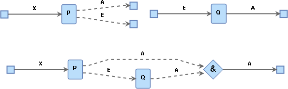
In this, the second option E of P is converted to the type of the first option A through Q. This fits the intuition of a recovery process that recovers from an exception E to produce an expected A. The result of the composition is a single A output, whether it came from P in the first place or from Q after "recovery".

If A gets connected to another process, whether the source will be P or Q is only determined at runtime. We therefore use the & merge node and label the output provenance to represent that the A output will be coming from this particular merge node.

In such cases we mark the provenance of the new output using & followed by the name of the composition that introduced the merge node.

Unused inputs and the : tag

When dealing with optional outputs, the JOIN action often needs to build buffers for unused inputs. See the standard example below:

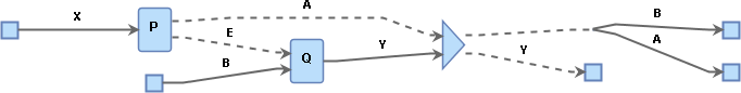
What should the output provenance for B be? Here it clearly should be Q. However, Q may not be atomic, but an intermediate composition instead. The reasoner does not know whether Q is composed of multiple components and which component B is coming from.

Mirroring the image above, here are 2 examples where Q is a composite process consisting of Q1 and Q2 (top) and Q3 and Q4 (bottom):

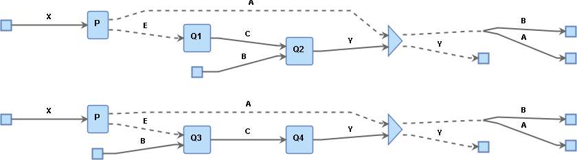
In the top case, B is an input of Q2, whereas in the bottom case B is an input of Q3. In both cases, the reasoner just sees an intermediate composition Q with inputs B and E and output Y as in the previous image. We therefore need a different way of tagging the provenance of B in a way that allows us to trace it back to Q2 or Q3.

This is accomplished by reporting the channel c of the unused input B. In the example above, the reasoner will produce a provenance leaf Q:c, i.e. the name of the (possibly composite) process Q followed by a colon : followed by the name of the channel of the unused input c.

The reasoner is effectively telling the graph interface to search in the process Q for an input with channel c and use the owner of that input as the source of B.

This may cause issues when multiple identical components introduce the same channel name multiple times in the same composition. The reasoner does not currently diambiguate between those because it does not even have that information.

Input Provenance

Each process can have multiple inputs, each with its own unique channel. This means we can generally track the owner of an input through the channel.

In our example above, NEG (C ⊕ D) of Q2 will have a unique channel name, let's assume cQ. When composing Q1 with Q2, this input is not affected. This means if we try to connect something to it, we already know cQ belongs to Q2 so we can track its provenance and connect the graph appropriately.

The composition actions only affect input channels in 2 ways:

1. The WITH action constructs new inputs that are options or merges of other inputs. These are reported in the composition step and their provenance is linked to the composite process, not its components.
2. The JOIN action manipulates inputs in order to match the output of the other (left) component. This includes adding buffers, using inputs from different components and merging options. In this case, we need to track the provenance of each part in the constructed input.

Back to our example, when composing P with Q, we connect NEG A with NEG (C ⊕ D) to create a new input NEG (A ⊗ (C ⊕ D)) that matches the output of P. At that point, we need to track that NEG A had some channel cP which can be traced back to P, whereas NEG (C ⊕ D) had channel cQ that we know belongs to Q. For this reason, we build the following provenance tree (shown next to the input parse tree), while ignoring the negation:

1⊗         ⊗
2|\        |\
3| \       | \
4A  ⊕      cP ⊕
5   |\        |\
6   | \       | \
7   C  D     cQ cQ

Note that the leaves of an input provenance tree, in principle, contain channels as opposed to those of an output provenance tree which contain process names.

There are a few particularities and special cases of leaves for input provenance, which we describe next.

Disambiguating same channels with a : tag

Assume a process Q with an input A ⊕ B on channel cQ. In the image shown below, we TENSOR Q with itself and then JOIN it with a process P with output (A ⊕ B) ⊗ (A ⊕ B):

As we are joining P to the the 2 Q processes, the reasoner will apply the par rule to compose the 2 A ⊗ B inputs into one that matches the output of P. Sticking to the explanation of input provenance we provided above, the input provenance for the composite input will be (cQ ⊕ cQ) ⊗ (cQ ⊕ cQ).

This would lead the graph engine to look for 4x cQ channels and fail because there are only 2 available, one for each instance of Q. The reasoner needs to somehow convey the information that the first 2 cQ channels in the provenance tree refer to the same channel, whereas the other 2 cQ channels refer to a single other channel.

This is accomplished by tagging each channel in the provenance tree with an integer. If 2 leaves in the provenance tree have the same channel and same number, they refer to the same, single channel. If hey have the same channel name, but a different number, they refer to 2 separate instances of that channel. Note that the actual number used has no other significance and is merely linked to an internal proof counter.

In our example, the reasoner will report an input provenance (cQ:4 ⊕ cQ:4) ⊗ (cQ:7 ⊕ cQ:7) (or some other numbers instead of 4 and 7). This is how the graph engine that generated the image above knew how to connect one A and one B to the top Q, corresponding to channel cQ:4, and the other A and the other B to the second Q, corresponding to channel cQ:7.

The # provenance

In some cases, an input being connected does not feed to any (atomic) process, but belongs to a buffer that is introduced. Such an input will be forwarded to the output of the composite process without change.

The reasoner reports the input provenance of such buffers using a hash # label for the leaf.

In our current composer implementation, we use a triangle "join" (or "terminator") node as a target to connect buffered resources to.

The & prefix

The issue of merged options in output provenance needs to be dealt with in input provenance too.

Let's revisit the same example:

As we are joining P and Q, the reasoner constructs an optional input A ⊕ E for Q using its existing input E and introducing a buffer of type A. Once the new input is constructed, we need to provide its input provenance. This must be such that E gets connected to Q, whereas A is connected to the merge node.

The reported input provenance is &_Step1 ⊕ cQ:5, where _Step1 the name of the composition, cQ the input channel of Q, and 5 some integer.

Future Work

Further clarifying and simplifying the provenance information is an obvious want for the future.

A few particularities exist because of the violation of channel uniqueness, so solving this problem in a more general way will help simplify provenance too.

Depending on further developments and needs of the frontend graph engine, we may extend provenance labels. The fact that the leaves can have any string as a label makes this structure very flexible and expandable.